Gallery
Reactive Transport in Porous Media
A coupled system combining linear combinations of conservation-law PDEs of chemical species \(e\) of the form $$ \partial_t n_e + \text{div} \Big( \mathbf{u}^{\alpha(e)} \Big) = T_e, $$ where \(\mathbf{u}^{\alpha(e)}\) is the velocity of the phase containing \(e\) and \(T_e\) is the source term (creation/consumption from chemical reactions), with nonlinear algebraic equations of the form $$ \prod_e n_e^{\gamma_{e,R}} = K_R, $$ for a given scalar \(K_R\), representing chemical reactions.
Numerical results: (gazeous CO2 injection)
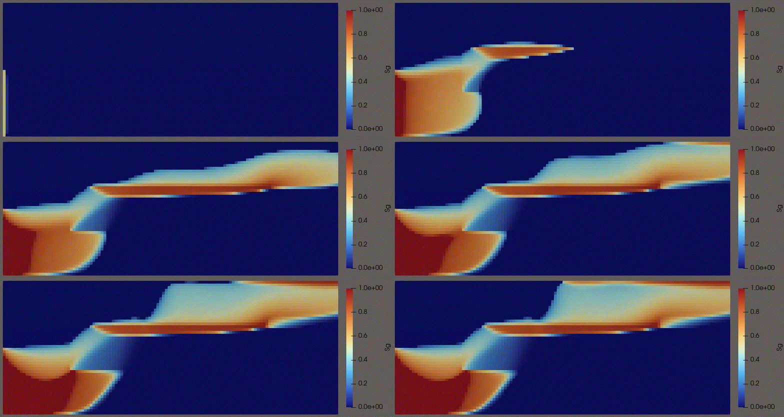
Gaz saturation.
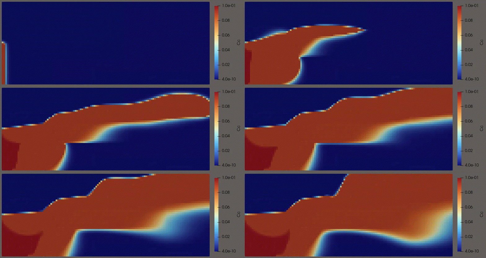
Fraction of gazeous CO2.
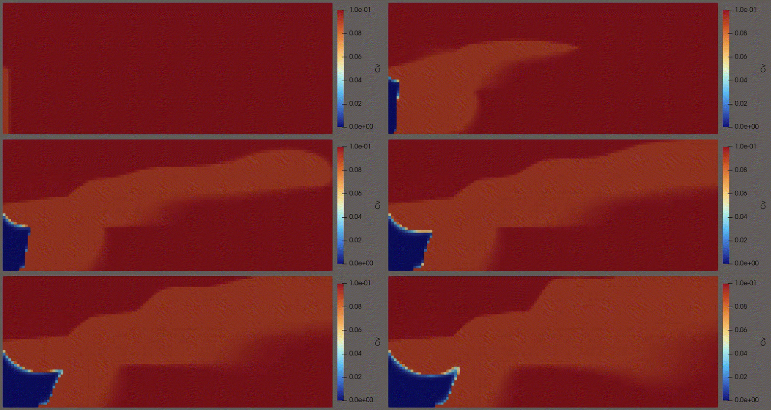
Fraction of gazeous H2O.
References:
- Fan Yaqing, Louis J. Durlofsky, and Hamdi A. Tchelepi. “A Fully-Coupled Flow-Reactive-Transport Formulation Based on Element Conservation, with Application to CO2 Storage Simulations.” Advances in Water Resources 42 (June 2012): 47–61.
- Ahusborde Etienne, Brahim Amaziane, Stephan De Hoop, et al. “A Benchmark Study on Reactive Two-Phase Flow in Porous Media: Part II - Results and Discussion.” Computational Geosciences 28, no. 3 (2024): 395–412.
Total Variation Denoising
We consider the Rudin-Osher-Fatemi model, $$ \min_{u\in BV(\Omega)\cap L^2(\Omega)} \frac{1}{2}\int_\Omega (u-f)^2\ dx + \alpha\int_\Omega |Du|. $$
Numerical results:
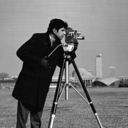
Original Image.
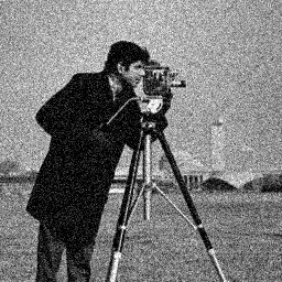
Noisy image \(f\).
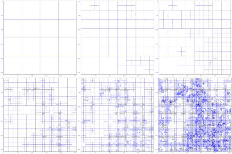
Mesh.
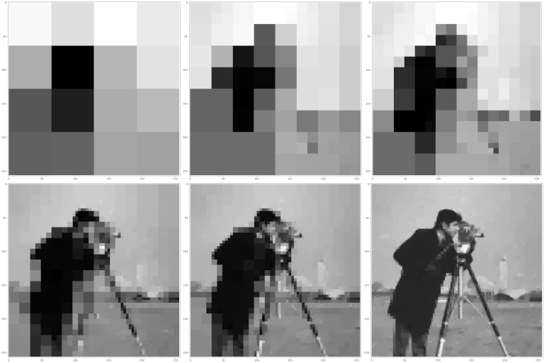
Solution \(u\).
References:
- Rudin, Leonid I., Stanley Osher, and Emad Fatemi. “Nonlinear Total Variation Based Noise Removal Algorithms.” Physica D: Nonlinear Phenomena 60, no. 1 (November 1, 1992): 259–68.
- Jacumin Thomas, and Andreas Langer. “An Adaptive Finite Difference Method for Total Variation Minimization.” Numerical Algorithms, ahead of print, March 19, 2025.
Image Inpainting
For \(t>0\), find \(u(t,\cdot)\) in \(H^1(D)\) such that, \begin{equation} \left\{\begin{array}{ll} \partial_t u(t,\cdot) - \Delta u(t,\cdot) = 0, & \text{in}\ D\setminus K, \\ u(t,\cdot) = f, & \text{in}\ K, \\ \frac{\partial u(t,\cdot)}{\partial \mathbf{n}} = 0, & \text{on}\ \partial D, \\ \end{array}\right . \end{equation} \[ u(0,\cdot) = \mathbf{1}_{K} f,\ \text{in}\ D. \]
Numerical results:
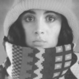
Original Image.
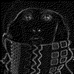
Inpainting Mask \(K\).
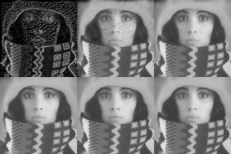
Solution \(u\) over time.
References:
- Marcelo Bertalmio, Guillermo Sapiro, Vincent Caselles, and Coloma Ballester. “Image inpainting”. In Proceedings of the 27th Annual Conference on Computer Graphics and Interactive Techniques, SIGGRAPH ’00, page 417–424, USA, 2000. ACM Press/Addison-Wesley Publishing Co..
- Belhachmi Zakaria, and Thomas Jacumin. “Optimal Interpolation Data for PDE-Based Compression of Images with Noise.” Communications in Nonlinear Science and Numerical Simulation 109 (June 2022): 106278.
Optical Flow
We consider the following optical flow estimation problem: $$ \left\{\begin{array}{ll} -\alpha \Delta u_1 + K_\rho\star(f_x)^2\ u_1 + K_\rho\star(f_x f_y)\ u_2 = - K_\rho\star(f_x f_t), & \text{in}\ [0,T]\times D, \\ -\alpha \Delta u_2 + K_\rho\star(f_y f_x)\ u_1 + K_\rho\star(f_y)^2\ u_2 = - K_\rho\star(f_y f_t), & \text{in}\ [0,T]\times D, \\ \frac{\partial u_1}{\partial\mathbf{n}} = \frac{\partial u_2}{\partial\mathbf{n}} = 0, & \text{on}\ [0,T]\times \partial D. \end{array}\right . $$
Numerical results: (Colors represent the directions of displacement)
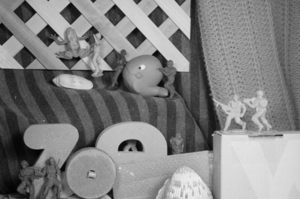
First Image \(f_1\).
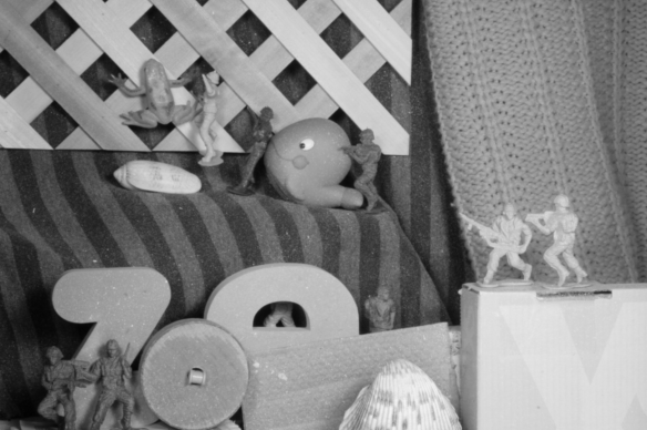
Second Image \(f_2\).
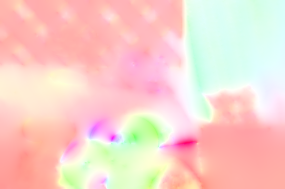
Optical Flow \(\mathbf{u}:=(u_1,u_2)\).
References:
- A. Bruhn, J. Weickert, and C. Schnörr, Lucas/Kanade Meets Horn/Schunck: Combining Local and Global Optic Flow Methods, International Journal of Computer Vision, 61 (2005), pp. 211–231.